Tutorial 1: A Detailed Quick Start Guide (DLPFC dataset)
This tutorial demonstrates the core functionalities of SEPAR (Spatial gene Expression PAttern Recognition) using the DLPFC (Dorsolateral Prefrontal Cortex) dataset. SEPAR is designed to identify spatial patterns in spatial transcriptomics data through graph-regularized matrix factorization.
Key Features
Spatial pattern identification
Pattern-specific gene detection
Spatially variable gene (SVG) identification
Gene expression refinement
Spatial domain clustering
Data Availability
The DLPFC dataset used in this tutorial can be accessed through multiple sources:
Dataset: The processed DLPFC data is hosted in the spatialLIBD repository
Manual Annotations: Expert-curated layer annotations are available in supplementary data folder from STAGATE[1]
import pandas as pd
import numpy as np
import scanpy as sc
import anndata as ad
import matplotlib.pyplot as plt
from sklearn.metrics import adjusted_rand_score
from sklearn.metrics.cluster import normalized_mutual_info_score as nmi
from SEPAR_model import SEPAR
Loading and Preparing Data
We’ll work with the DLPFC dataset. Here’s how to load and prepare the data:
# Define parameters for the specific slice
slice_idx = 151507
algorithm_params = {
    "151507": {"nslt": 3000, "alpha": 0.7, "l1": 0.01, "lam": 0.3}
}
params = algorithm_params.get(str(slice_idx), {})

# Load annotation data
anno_df = pd.read_csv('dataset/DLPFC/barcode_level_layer_map.tsv', sep='\t', header=None)

# Read Visium data
adata = sc.read_visium(path="dataset/DLPFC//%d" % slice_idx,
                      count_file="%d_filtered_feature_bc_matrix.h5" % slice_idx)
adata.var_names_make_unique()

# Process annotations
anno_df1 = anno_df.iloc[anno_df[1].values.astype(str) == str(slice_idx)]
anno_df1.columns = ["barcode", "slice_id", "layer"]
anno_df1.index = anno_df1['barcode']
adata.obs = adata.obs.join(anno_df1, how="left")
adata = adata[adata.obs['layer'].notna()]

# Initialize SEPAR
n_cluster = len(adata.obs['layer'].unique())
separ = SEPAR(adata.copy(), n_cluster=n_cluster)
separ.adata.obs['Region'] = separ.adata.obs['layer']
Data Preprocessing
SEPAR includes several preprocessing steps:
# Preprocess the data
separ.preprocess(min_cells=40, n_top_genes=6000)
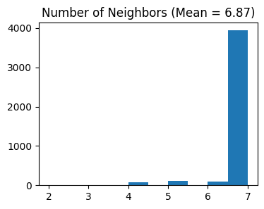
# Compute spatial graph
separ.compute_graph()
# Select features using Moran's I
separ.select_morani(nslt=params['nslt'])
# Compute weights
separ.compute_weight(n_cluster=n_cluster)
After filtering: (4221, 12597)
Counting moran's i ...

Finish selecting
Parameters Explanation:
min_cells: Minimum number of cells required for a gene to be consideredn_top_genes: Number of highly variable genes to selectnslt: Number of spatially variable genes to select using Moran’s I statisticn_cluster: Number of expected spatial domains/clusters
1. Running SEPAR Algorithm
# Run SEPAR algorithm
separ.separ_algorithm(
    r=30,              # Number of spatial patterns
    alpha=0.7,         # Graph regularization weight
    beta=0.01,         # Sparsity penalty weight (previously l1)
    gamma=0.3          # Pattern orthogonality weight (previously lam)
)
Processing iterations: 100%|██████████| 100/100 [00:24<00:00, 4.03it/s]
Parameters Explanation:
r: IntegerNumber of spatial patterns to identify
alpha: FloatWeight for graph regularization term
Controls spatial smoothness of patterns
Typical range: 0.1-1.0
beta: Float (previously l1)Weight for sparsity penalty
Controls pattern distinctness and localization
Typical range: 0.01-0.1
gamma: Float (previously lam)Weight for pattern orthogonality term
Controls redundancy between patterns
Typical range: 0.1-1.0
Results:
separ.Wpn: Spatial patterns matrix (W in the paper)separ.Hpn: Gene loading matrix (H in the paper)separ.err_list: Reconstruction errors during optimization
2. Identifying Pattern-Specific Genes
# Identify pattern-specific genes
pattern_genes = separ.identify_pattern_specific_genes(
    n_patterns=30,    # Number of patterns to consider
    threshold=0.3     # Threshold for gene-pattern association
)
Parameters Explanation:
n_patterns: Integer (default=30)Number of top patterns to analyze
Should be less than or equal to total patterns from decomposition
threshold: Float (default=0.3)Threshold for determining pattern-specific genes
Higher values yield more stringent gene selection
Results Storage:
self.pattern_specific_mask: List of boolean arraysLength equals to
n_patternsEach array indicates which genes are specific to that pattern
self.genes_per_pattern: Number of specific genes per patternself.Wpnn,self.Hpnn: Normalized pattern and gene loading matrices
Return:
pattern_genes: List of listsLength equals to
n_patternsEach sublist contains genes specific to that pattern
Genes are sorted by specificity score
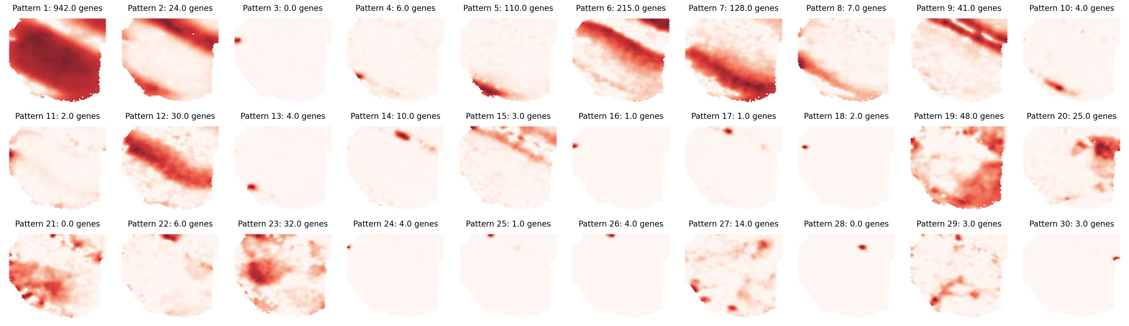
Pattern Visualization and Pattern-specific Genes
First, let’s visualize the identified spatial patterns and analyze their characteristics:
# Visualize all spatial patterns
sim_slt = separ.sim_res(separ.Wpn, separ.Hpn, separ.Xt.T)
sim_argsort = np.argsort(-sim_slt)

num_patterns = 30
plt.figure(dpi=200, figsize=(24, 7))
for i in range(30):
    ii = sim_argsort[i]
    plt.subplot(3, np.int32(num_patterns/3), i + 1)
    plt.scatter(separ.loc[:, 0], -separ.loc[:, 1],
                c=separ.Wpn[:, ii].reshape(-1, 1),
                s=1.2, cmap='Reds')
    plt.axis('off')
    plt.title(f'Pattern {i + 1}: {separ.genes_per_pattern[ii]} genes',
              fontsize=12)
plt.tight_layout()
plt.show()
# Create and display sorted pattern-specific genes table
print("\nTop Pattern-Specific Genes (Sorted by Pattern Significance):")
print("-" * 100)
print(f"{'Pattern':11} | {'Significance':11} | {'#Genes':8} | {'Top Genes'}")
print("-" * 100)

for rank, pattern_idx in enumerate(sim_argsort[:30]):
    genes = pattern_genes[pattern_idx]
    if len(genes) == 0:
        gene_str = "None"
    else:
        gene_str = ", ".join(genes[:10])
        if len(genes) > 10:
            gene_str += "..."

    print(f"Pattern {rank+1:<3} | {sim_slt[pattern_idx]:.4f}      | {len(genes):<8} | {gene_str}")
print("-" * 100)
Top Pattern-Specific Genes (Sorted by Pattern Significance):
----------------------------------------------------------------------------------------------------
Pattern     | Significance | #Genes   | Top Genes
----------------------------------------------------------------------------------------------------
Pattern 1   | 0.9418      | 942      | ATP1A3, HINT1, UCHL1, CISD1, VGF, CHCHD10, TUBB2A, NDUFA4, COX4I1, SNAP25...
Pattern 2   | 0.8872      | 24       | GFAP, GALNT15, CST3, APLNR, MT-ND2, MT-ND1, MT3, MT-ATP6, MT-ND4, MT-CYB...
Pattern 3   | 0.7692      | 0        | None
Pattern 4   | 0.7480      | 6        | LTB, CCL19, TACSTD2, PIGB, RLBP1, IRF7
Pattern 5   | 0.7298      | 110      | LDB3, GJB1, ERMN, GLDN, NKX6-2, PLEKHH1, ANLN, AQP1, CARNS1, FAM222A...
Pattern 6   | 0.6737      | 215      | LINC00507, NEUROD1, NEK2, CALB1, EFCAB1, FFAR4, LRRTM4, SHISA8, PENK, KCNA4...
Pattern 7   | 0.6705      | 128      | TRABD2A, LRMP, FEZF2, TSHZ2, PCP4, GAL, SMYD2, MKX, HS3ST2, CLSTN2...
Pattern 8   | 0.6345      | 7        | NR4A2, KRT17, NTNG2, THEMIS, SEMA3E, CTGF, TMEM233
Pattern 9   | 0.6290      | 41       | RELN, MT1H, RGR, F3, MSX1, MT1F, GSTM5, HEPN1, IQCK, FABP7...
Pattern 10  | 0.6217      | 4        | ZMYND10, AC004233.3, LAIR1, BIK
Pattern 11  | 0.6013      | 2        | SSTR3, TSHZ2
Pattern 12  | 0.5910      | 30       | SHD, TPBG, NEFH, NEFM, VAMP1, CPB1, KCNS1, NEUROD6, SYT2, GRM7...
Pattern 13  | 0.5670      | 4        | ADAMTS1, NRIP2, TNFRSF12A, TMEM233
Pattern 14  | 0.5600      | 10       | MYH11, AC073896.2, AC105942.1, ANXA3, ACTA2, APLNR, MYL9, ARRDC4, TUT7, AL031056.1
Pattern 15  | 0.5556      | 3        | CEP76, MN1, C1QL2
Pattern 16  | 0.5473      | 1        | PTER
Pattern 17  | 0.5029      | 1        | DPY19L3
Pattern 18  | 0.4962      | 2        | TMC7, NAGA
Pattern 19  | 0.4912      | 48       | CEACAM6, CYP2A6, SCGB2A1, TFF1, CLEC3A, CYP4Z1, SCGB1D2, TPRG1, AZGP1, AGR2...
Pattern 20  | 0.4788      | 25       | CIDEC, G0S2, PLIN1, FABP4, THRSP, ADH1B, PLIN4, ADIPOQ, SAA1, SAA2...
Pattern 21  | 0.4665      | 0        | None
Pattern 22  | 0.4591      | 6        | S100G, ALB, MGP, AC007952.4, GPC3, LTBP2
Pattern 23  | 0.4514      | 32       | IER3, CPB1, BAMBI, CGA, PSMB9, CLDN7, CTPS2, H2AFJ, RAB11FIP1, HK2...
Pattern 24  | 0.4493      | 4        | NOSTRIN, LYPD6B, ERFE, ACP6
Pattern 25  | 0.4292      | 1        | PEBP4
Pattern 26  | 0.4059      | 4        | PRR15L, ALB, PRR15, TRPV3
Pattern 27  | 0.3753      | 14       | JCHAIN, IGHA1, IGLC2, IGHM, IGLC3, IGHA2, IGKC, KRT15, IGHG3, IGHG1...
Pattern 28  | 0.3605      | 0        | None
Pattern 29  | 0.3521      | 3        | HBB, HBA2, HBA1
Pattern 30  | 0.3486      | 3        | ZNF446, TRARG1, OTUB2
----------------------------------------------------------------------------------------------------
3. Spatially Variable Genes (SVGs) Analysis
# Get SVG results
svg_results = separ.recognize_svgs(err_tol=0.7)
svg_results
{'svgs': Index(['SCGB2A2', 'SCGB1D2', 'GFAP', 'MBP', 'MT-CO2', 'MT-CO1', 'MT-ND1',
        'SAA1', 'MT-ATP6', 'MT-ND2',
        ...
        'SLC25A46', 'MAP7D1', 'LIMCH1', 'TCF25', 'DCTN2', 'CAMSAP2', 'ARL2',
        'SPAG9', 'CFL2', 'TCAF1'],
       dtype='object', length=1831),
 'gene_ranking': array([   4,    5,   19, ..., 2149,  935, 2008]),
 'error_rates': array([0.13682987, 0.20417668, 0.22127199, ..., 0.88352493, 0.6206503 ,
        0.90467464])}
Parameters Explanation:
err_tol: Float, default=0.7Error tolerance threshold for SVG identification
Controls which genes are classified as spatially variable based on reconstruction error
Results Storage:
svg_results['svgs']: Names of identified spatially variable genessvg_results['gene_ranking']: Indices of all genes sorted by spatial variability (ascending error rates)svg_results['error_rates']: Reconstruction error rates for each gene
Let’s visualize some top and bottom SVGs:
gene_ranking = svg_results['gene_ranking']
# Create a single figure with subplots for top SVGs and bottom non-SVGs
plt.figure(figsize=(8.5, 5), dpi=100)
plt.rcParams['font.size'] = 8
# Plot top 3 SVGs
for i in range(3):
    plt.subplot(2, 3, i+1)
    gene_idx = gene_ranking[i]
    gene_name = adata.var_names[gene_idx]
    gene_exp = separ.adata[:, gene_idx].X.toarray().flatten()

    scatter = plt.scatter(separ.adata.obsm['spatial'][:, 0],
                        -separ.adata.obsm['spatial'][:, 1],
                        c=gene_exp, s=5, cmap='Reds')
    plt.title(f'Top SVG {i+1}: {gene_name}')
    plt.axis('off')
    plt.colorbar(scatter)

# Plot bottom 3 non-SVGs
for i in range(3):
    plt.subplot(2, 3, i+4)
    gene_idx = gene_ranking[-(i+1)]
    gene_name = adata.var_names[gene_idx]
    gene_exp = separ.adata[:, gene_idx].X.toarray().flatten()

    scatter = plt.scatter(separ.adata.obsm['spatial'][:, 0],
                        -separ.adata.obsm['spatial'][:, 1],
                        c=gene_exp, s=5, cmap='Reds')
    plt.title(f'Bottom non-SVG {i+1}: {gene_name}')
    plt.axis('off')
    plt.colorbar(scatter)

plt.tight_layout()
plt.show()

4. Gene Expression Refinement
adata_refined = separ.get_refined_expression()
Returns:
adata_refined: AnnData objectContains denoised gene expression matrix
Preserves original gene names and spot indices from input AnnData
.X: Stores the refined expression matrix
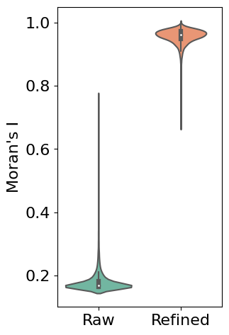
Evaluating Refinement Performance
First, we use Moran’s I statistic to quantitatively evaluate the improvement in spatial patterns. Moran’s I measures spatial autocorrelation, with higher values indicating stronger spatial patterns. The violin plot below compares the distribution of Moran’s I values between raw and refined expression data across all genes:
# Calculate Moran's I for both raw and refined data
morani = sc.metrics.morans_i(separ.adata)
morani_refine = sc.metrics.morans_i(adata_refined)

# Create DataFrame for violin plot
data_violin = pd.DataFrame({
    'Moran\'s I': np.concatenate([morani, morani_refine]),
    'Condition': ['Raw'] * len(morani) + ['Refined'] * len(morani_refine)
})

import seaborn as sns
# Create violin plot
plt.rcParams['font.size'] = 16
plt.figure(figsize=(3, 5.5))
sns.violinplot(x='Condition', y='Moran\'s I', data=data_violin, palette='Set2')
plt.ylabel('Moran\'s I')
plt.xlabel('')
plt.show()
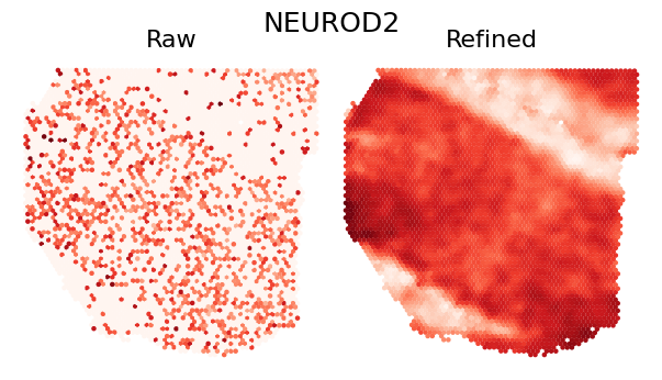
Single Gene Visualization
To demonstrate the refinement effect at individual gene level, we visualize the spatial expression pattern of a single gene. The comparison shows how SEPAR preserves and enhances genuine spatial patterns while reducing technical noise:
def plot_gene_refinement(gene_name, separ, adata_refined):
    """
    Visualize raw and refined expression patterns for a specific gene.

    Parameters
    ----------
    gene_name : str
        Name of the gene to visualize
    separ : SEPAR object
        SEPAR object containing raw data
    adata_refined : AnnData
        Refined expression data from get_refined_expression()
    """
    # Get gene index and expression values
    gene_idx = separ.adata.var_names.get_loc(gene_name)
    raw_exp = separ.adata[:, gene_idx].X.toarray().flatten()
    refined_exp = adata_refined.X[:, gene_idx]

    # Create comparison plot
    plt.rcParams['font.size'] = 16
    plt.figure(dpi=100, figsize=(7/1.2, 4/1.2))

    # Set main title
    plt.suptitle(gene_name, fontsize=18)

    # Plot raw expression
    plt.subplot(1, 2, 1)
    plt.scatter(separ.loc[:, 0], -separ.loc[:, 1],
                c=raw_exp, s=5, cmap='Reds', rasterized=True)
    plt.axis('off')
    plt.title('Raw', fontsize=16)

    # Plot refined expression
    plt.subplot(1, 2, 2)
    plt.scatter(separ.loc[:, 0], -separ.loc[:, 1],
                c=refined_exp, s=5, cmap='Reds', rasterized=True)
    plt.axis('off')
    plt.title('Refined', fontsize=16)

    plt.tight_layout(pad=0)
    plt.show()

plot_gene_refinement("NEUROD2", separ, adata_refined)
plot_gene_refinement("MBP", separ, adata_refined)

plot_gene_refinement("GFAP", separ, adata_refined)

5. Performing Clustering
# Perform clustering
cluster_res = separ.clustering(n_cluster=n_cluster, N1=30-n_cluster-7, N2=5)
Parameters Explanation:
n_cluster: IntegerNumber of spatial domains to identify
N1: Integer, optionalNumber of patterns to retain after l2-norm filtering
Default: r - 5 - n_cluster (where r is the total number of patterns)
N2: Integer, default=3Number of patterns to retain after Pattern Specificity Score (PSS) filtering
Default value is 3 as specified in the paper
Results Storage:
self.labelres: Array of cluster labels for each spotself.adata.obs['clustering']: Cluster assignments stored in AnnData object
Clustering Results Visualization
Compare the manual annotation with SEPAR clustering results:
# Calculate clustering metrics
Y_list = separ.adata.obs['Region']
Ari = adjusted_rand_score(Y_list, separ.labelres)
Nmi = nmi(Y_list, separ.labelres)

# Create visualization
fig, axs = plt.subplots(1, 2, figsize=(12, 6), dpi = 50)
plt.rcParams['font.size'] = 12
# Manual annotation plot
groups = separ.adata.obs['Region'].astype('str')
unique_regions = groups.unique()
region_to_num = {region: num for num, region in enumerate(unique_regions)}
groups = separ.adata.obs['Region'].map(region_to_num)

scatter = axs[0].scatter(separ.loc[:, 0], -separ.loc[:, 1],
                        c=groups, s=10, cmap='tab10')
axs[0].set_title("Manual annotation", fontsize=15)
axs[0].axis('off')
legend = axs[0].legend(*scatter.legend_elements(),
                      title="Layers",
                      bbox_to_anchor=(0.95, 0.5),
                      loc='center left')

# SEPAR clustering plot
scatter = axs[1].scatter(separ.loc[:, 0], -separ.loc[:, 1],
                        c=separ.labelres, s=10, cmap='Set1')
axs[1].set_title(f"SEPAR clustering (ARI = {Ari:.3f}, NMI = {Nmi:.3f})",
                 fontsize=15)
axs[1].axis('off')

plt.tight_layout()
plt.show()

References
[1] Dong, Kangning, and Shihua Zhang. “Deciphering spatial domains from spatially resolved transcriptomics with an adaptive graph attention auto-encoder.” Nature Communications 13.1 (2022): 1-12.