Tutorial 5: multi-slice analysis (DLPFC dataset)
Data Availability
The DLPFC dataset used in this tutorial can be accessed through multiple sources:
Dataset: The processed DLPFC data is hosted in the spatialLIBD repository
Manual Annotations: Expert-curated layer annotations are available in supplementary data folder from STAGATE[1]
Introduction
SEPARmult extends the original SEPAR algorithm to handle multiple tissue sections simultaneously, enabling:
Joint pattern discovery across sections
Consistent spatial domain identification
Cross-section gene program analysis
Integrated refinement of gene expression
Data Preparation
First, let’s import the necessary packages and load the data:
import pandas as pd
import numpy as np
import scanpy as sc
import anndata as ad
import matplotlib.pyplot as plt
from SEPARmult_model import SEPARmult

# Load multiple slices
section_ids = ['151673','151674','151675','151676']
Batch_list = []

# Load annotation data
anno_df = pd.read_csv('dataset/DLPFC/barcode_level_layer_map.tsv', sep='\t', header=None)

for section_id in section_ids:
    # Read Visium data
    adata = sc.read_visium(path="dataset/DLPFC/%s" % section_id,
                          count_file="%s_filtered_feature_bc_matrix.h5" % section_id)

    # Add layer annotations
    anno_df1 = anno_df.iloc[anno_df[1].values.astype(str) == str(section_id)]
    anno_df1.columns = ["barcode", "slice_id", "layer"]
    anno_df1.index = anno_df1['barcode']
    adata.obs = adata.obs.join(anno_df1, how="left")

    # Filter spots with no annotation
    adata = adata[adata.obs['layer'].notna()]
    adata.obs['Ground Truth'] = adata.obs['layer'].astype('category')

    # Make spot names unique
    adata.obs_names = [x+'_'+section_id for x in adata.obs_names]

    Batch_list.append(adata)

# Initialize SEPARmult
separ = SEPARmult(Batch_list, section_ids, n_cluster=7)
<frozen importlib._bootstrap>:219: RuntimeWarning: scipy._lib.messagestream.MessageStream size changed, may indicate binary incompatibility. Expected 56 from C header, got 64 from PyObject
Data Preprocessing
SEPARmult requires several preprocessing steps to ensure data quality and compatibility across sections:
# Basic filtering and normalization
separ.preprocess(min_cells=50, normalize=True)

# Filter to keep only shared genes across sections
separ.filter_shared_genes()

# Compute spatial graphs for each section
separ.compute_graph(radius_rate=1.3)

# Select highly variable genes using Moran's I
separ.select_morani(nslt=3000)

# Concatenate data and compute weights
separ.concat_data()
separ.compute_weight(n_cluster=7)
After filtering and preprocessing: (3611, 13080)
After filtering and preprocessing: (3635, 13968)
After filtering and preprocessing: (3566, 12443)
After filtering and preprocessing: (3431, 12577)
Number of shared genes: 12264
Mean number of neighbors for sample 151673: 6.83
Mean number of neighbors for sample 151674: 6.81
Mean number of neighbors for sample 151675: 6.80
Mean number of neighbors for sample 151676: 6.82
Moran's I selection finished
Data concatenation finished
Running SEPARmult Algorithm
The core algorithm integrates information across all sections to identify spatial patterns:
# Run SEPARmult algorithm
separ.separ_algorithm(
    r=30,              # Number of spatial patterns
    alpha=0.5,         # Graph regularization weight
    beta=0.003,         # Sparsity penalty weight
    gamma=0.5,          # Pattern orthogonality weight
)
Processing iterations: 100%|██████████| 100/100 [01:50<00:00, 1.10s/it]
Pattern-Specific Gene Identification
SEPARmult can identify genes specific to each spatial pattern:
# Identify pattern-specific genes
pattern_genes = separ.identify_pattern_specific_genes(
    n_patterns=30,    # Number of patterns to analyze
    threshold=0.3      # Threshold for gene specificity
)
Number of SVGs identified: 1519
Visualization of Patterns with Pattern-Specific Genes
# Visualize patterns across all sections
sim_slt = separ.sim_res(separ.Wpn, separ.Hpn, separ.Xt.T)
sim_argsort = np.argsort(-sim_slt)

num_patterns = 30
for j, adata in enumerate(separ.adata_list):
    batch_name = str(151673 + j)
    loc = adata.obsm['spatial']

    plt.figure(dpi=80, figsize=(20, 7))
    for i in range(30):
        ii = sim_argsort[i]
        plt.subplot(3, np.int32(num_patterns/3), i + 1)

        # Get indices for current section
        batch_indices = separ.adata_concat.obs['batch_name'] == batch_name

        plt.scatter(
            loc[:, 0],
            -loc[:, 1],
            c=separ.Wpn[batch_indices, ii].reshape(-1, 1),
            s=1.2,
            cmap='Reds'
        )
        plt.axis('off')
        plt.title(
            f'Pattern {i + 1}\n{int(separ.genes_per_pattern[ii])} genes',
            fontsize=12
        )
    plt.suptitle(f'Section {batch_name}', fontsize=16, y=1.02)
    plt.tight_layout()
    plt.show()


# Create comprehensive pattern-gene table
print("\nPattern Analysis Summary (Sorted by Pattern Significance):")
print("-" * 120)
print(f"{'Pattern':8} | {'Significance':11} | {'#Genes':8} | {'Top Genes'}")
print("-" * 120)


# Print detailed pattern information
for rank, pattern_idx in enumerate(sim_argsort[:30]):
    genes = pattern_genes[pattern_idx]
    if len(genes) == 0:
        gene_str = "None"
    else:
        gene_str = ", ".join(genes[:5])
        if len(genes) > 5:
            gene_str += "..."

    print(
        f"Pattern {rank+1:<2} | "
        f"{sim_slt[pattern_idx]:.4f}      | "
        f"{len(genes):<8} | "
        f"{gene_str}"
    )
print("-" * 120)
Pattern Analysis Summary (Sorted by Pattern Significance):
------------------------------------------------------------------------------------------------------------------------
Pattern  | Significance | #Genes   | Top Genes
------------------------------------------------------------------------------------------------------------------------
Pattern 1  | 0.9283      | 790      | BEX1, TPI1, SNRPN, SNAP25, MDH1...
Pattern 2  | 0.8234      | 0        | None
Pattern 3  | 0.8032      | 369      | AC096564.1, AQP1, LPAR1, MOBP, CTNNA3...
Pattern 4  | 0.7088      | 0        | None
Pattern 5  | 0.7042      | 1        | HEPN1
Pattern 6  | 0.6815      | 0        | None
Pattern 7  | 0.6577      | 230      | FREM3, LINC02552, CALB1, CARTPT, CUX2...
Pattern 8  | 0.6533      | 23       | THEMIS, OLFML2B, SEMA3E, SMIM32, NR4A2...
Pattern 9  | 0.6470      | 0        | None
Pattern 10 | 0.6413      | 0        | None
Pattern 11 | 0.6405      | 87       | TP53TG5, DNAH17, CAHM, SLC35D2, NINJ2...
Pattern 12 | 0.6347      | 0        | None
Pattern 13 | 0.6138      | 9        | MSX1, MT1H, FABP7, LIX1, AGT...
Pattern 14 | 0.6096      | 2        | CD52, S100A4
Pattern 15 | 0.6072      | 0        | None
Pattern 16 | 0.6020      | 10       | RELN, DACT1, PENK, C1QL2, MUC19...
Pattern 17 | 0.5990      | 49       | PLCH1, GAL, RORB, SYT2, PVALB...
Pattern 18 | 0.5934      | 23       | TRABD2A, FEZF2, GRIN3A, PCP4, HS3ST2...
Pattern 19 | 0.5799      | 6        | NTNG1, GPR6, COL5A2, CTXN3, GPX3...
Pattern 20 | 0.5784      | 9        | MYH11, ACTA2, ADAMTS1, MYL9, TPM2...
Pattern 21 | 0.5177      | 0        | None
Pattern 22 | 0.4799      | 42       | FCGBP, MMP11, GFRA1, AGR2, CISH...
Pattern 23 | 0.4731      | 41       | CPB1, CGA, CSTA, RAB11FIP1, CNTD2...
Pattern 24 | 0.4268      | 35       | SCGB2A1, SCGB1D2, CYP4Z1, CEACAM6, SCGB2A2...
Pattern 25 | 0.4190      | 0        | None
Pattern 26 | 0.3858      | 8        | IGHG1, IGHG3, IGHG4, IGLC3, IGLC2...
Pattern 27 | 0.3704      | 8        | JCHAIN, IGHA2, IGHA1, KRT15, IGLC2...
Pattern 28 | 0.3668      | 14       | SAA2, CIDEC, G0S2, SAA1, FABP4...
Pattern 29 | 0.3077      | 2        | MGP, S100G
Pattern 30 | 0.2468      | 3        | HBB, HBA1, HBA2
------------------------------------------------------------------------------------------------------------------------
Spatially Variable Genes (SVGs) Analysis
# Identify spatially variable genes
svg_results = separ.recognize_svgs(err_tol=0.5)

# Extract results
svgs = svg_results['svgs']
gene_ranking = svg_results['gene_ranking']
error_rates = svg_results['error_rates']

print(f"Number of SVGs identified: {len(svgs)}")
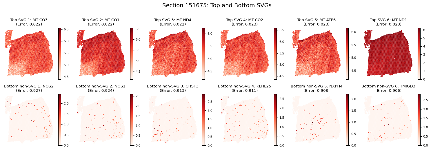
Visualizing Spatially Variable Genes
Let’s visualize some examples of the most and least spatially variable genes across sections:
# Visualize SVGs for each section
for j, adata in enumerate(separ.adata_list):
    batch_name = str(151673 + j)
    loc = adata.obsm['spatial']

    plt.figure(figsize=(15, 5), dpi=100)
    plt.suptitle(f'Section {batch_name}: Top and Bottom SVGs', y=1.02, fontsize=14)
    plt.rcParams['font.size'] = 8

    # Plot top 6 SVGs
    for i in range(6):
        plt.subplot(2, 6, i+1)
        gene_idx = gene_ranking[i]
        gene_name = separ.adata_concat.var_names[gene_idx]
        gene_exp = adata[:, gene_idx].X.toarray().flatten()

        scatter = plt.scatter(
            loc[:, 0],
            -loc[:, 1],
            c=gene_exp,
            s=1,
            cmap='Reds'
        )
        plt.title(f'Top SVG {i+1}: {gene_name}\n(Error: {error_rates[gene_idx]:.3f})')
        plt.axis('off')
        plt.colorbar(scatter)

    # Plot bottom 6 non-SVGs
    for i in range(6):
        plt.subplot(2, 6, i+7)
        gene_idx = gene_ranking[-(i+1)]
        gene_name = separ.adata_concat.var_names[gene_idx]
        gene_exp = adata[:, gene_idx].X.toarray().flatten()

        scatter = plt.scatter(
            loc[:, 0],
            -loc[:, 1],
            c=gene_exp,
            s=1,
            cmap='Reds'
        )
        plt.title(f'Bottom non-SVG {i+1}: {gene_name}\n(Error: {error_rates[gene_idx]:.3f})')
        plt.axis('off')
        plt.colorbar(scatter)

    plt.tight_layout()
    plt.show()


Gene Expression Refinement
# Get refined expression data
adata_refined = separ.get_refined_expression()
Single Gene Visualization
def plot_gene_refinement_multi(gene_name, separ, adata_refined):
    """
    Visualize raw and refined expression patterns across all sections.
    """
    plt.figure(figsize=(12, 5))
    plt.suptitle(f'Expression Patterns of {gene_name}', fontsize=16, y=1.05)

    for i, adata in enumerate(separ.adata_list):
        batch_name = str(151673 + i)
        batch_mask = separ.adata_concat.obs['batch_name'] == batch_name
        loc = adata.obsm['spatial']

        # Get gene expression values
        gene_idx = adata.var_names.get_loc(gene_name)
        raw_exp = adata[:, gene_idx].X.toarray().flatten()
        refined_exp = adata_refined[batch_mask, gene_idx].X

        # Plot raw expression
        plt.subplot(2, 4, i + 1)
        scatter = plt.scatter(
            loc[:, 0],
            -loc[:, 1],
            c=raw_exp,
            s=1,
            cmap='Reds',
            rasterized=True
        )
        plt.axis('off')
        plt.title(f'Section {batch_name} - Raw')
        plt.colorbar(scatter)

        # Plot refined expression
        plt.subplot(2, 4, i + 5)
        scatter = plt.scatter(
            loc[:, 0],
            -loc[:, 1],
            c=refined_exp,
            s=1,
            cmap='Reds',
            rasterized=True
        )
        plt.axis('off')
        plt.title(f'Section {batch_name} - Refined')
        plt.colorbar(scatter)

    plt.tight_layout()
    plt.show()

# Visualize example genes
example_genes = ["TRABD2A","CPB1", "MBP", "GFAP", "JCHAIN", "SAA2"]
for gene in example_genes:
    plot_gene_refinement_multi(gene, separ, adata_refined)


Performing Clustering
# Perform clustering
labels = separ.clustering(
    n_cluster=7,       # Number of spatial domains
    N1=13,     # Range for norm-based filtering
    N2=5       # Range for similarity-based filtering
)


# Distribute clustering results back to individual sections
clustering_results = separ.adata_concat.obs['clustering']
batch_info = separ.adata_concat.obs['batch_name']

for i, adata in enumerate(separ.adata_list):
    # Get batch name for current section
    batch_name = str(151673 + i)

    # Extract cells belonging to current section
    section_cells = batch_info[batch_info == batch_name].index

    # Get clustering results for current section
    section_clustering = clustering_results.loc[section_cells]

    # Store clustering results in original AnnData object
    adata.obs['clustering'] = section_clustering

# Calculate clustering accuracy (if ground truth available)
from sklearn.metrics import adjusted_rand_score
ARI_list = []
for bb in range(4):
    ARI = adjusted_rand_score(
        Batch_list[bb].obs['Ground Truth'],
        Batch_list[bb].obs['clustering']
    )
    ARI_list.append(round(ARI, 2))
print("ARI scores for each section:", ARI_list)
ARI scores for each section: [0.58, 0.56, 0.53, 0.53]
Clustering Results Visualization
from sklearn.metrics.cluster import normalized_mutual_info_score
# Calculate ARI and NMI scores for each section
ARI_list = []
NMI_list = []
for i, adata in enumerate(separ.adata_list):
    ARI = adjusted_rand_score(
        adata.obs['Ground Truth'],
        adata.obs['clustering']
    )
    NMI = normalized_mutual_info_score(
        adata.obs['Ground Truth'],
        adata.obs['clustering']
    )
    ARI_list.append(ARI)
    NMI_list.append(NMI)

# Create visualization with 2x4 subplots
fig, axs = plt.subplots(2, 4, figsize=(20, 10), dpi=100)
plt.rcParams['font.size'] = 12

for i, adata in enumerate(separ.adata_list):
    batch_name = str(151673 + i)
    loc = adata.obsm['spatial']

    # Ground truth plot (top row)
    groups = adata.obs['Ground Truth'].astype('str')
    unique_regions = groups.unique()
    region_to_num = {region: num for num, region in enumerate(unique_regions)}
    groups = adata.obs['Ground Truth'].map(region_to_num)

    scatter = axs[0, i].scatter(
        loc[:, 0],
        -loc[:, 1],
        c=groups,
        s=10,
        cmap='tab10'
    )
    axs[0, i].set_title(f"Section {batch_name}\nManual annotation", fontsize=12)
    axs[0, i].axis('off')

    # Add legend to the first plot only
    if i == 0:
        legend = axs[0, i].legend(
            *scatter.legend_elements(),
            title="Layers",
            bbox_to_anchor=(1.05, 1),
            loc='upper left'
        )

    # SEPAR clustering plot (bottom row)
    cluster_labels = adata.obs['clustering'].astype(int).values

    scatter = axs[1, i].scatter(
        loc[:, 0],
        -loc[:, 1],
        c=cluster_labels,
        s=10,
        cmap='Set1'
    )

    axs[1, i].set_title(
        f"SEPAR clustering\nARI = {ARI_list[i]:.3f}, NMI = {NMI_list[i]:.3f}",
        fontsize=12
    )
    axs[1, i].axis('off')

plt.suptitle('SEPAR Clustering Results Across Sections', fontsize=16, y=1.02)
plt.tight_layout()
plt.show()

print("\nMetrics for each section:")
print("-" * 50)
print(f"{'Section':10} | {'ARI':10} | {'NMI':10}")
print("-" * 50)
for i in range(len(ARI_list)):
    print(f"{151673+i:<10} | {ARI_list[i]:10.3f} | {NMI_list[i]:10.3f}")

Metrics for each section:
--------------------------------------------------
Section    | ARI        | NMI
--------------------------------------------------
151673     |      0.578 |      0.729
151674     |      0.564 |      0.713
151675     |      0.533 |      0.671
151676     |      0.528 |      0.683