Tutorial 2: mouse olfactory bulb generated by Stereo-seq
This tutorial demonstrates the analysis of spatial transcriptomics data from the mouse olfactory bulb, generated using Stereo-seq technology. The dataset is publicly available through Zenodo.
For quality control purposes, we preprocessed the data by filtering out spots located outside the main tissue region following the STAGATE method[1]. The curated dataset containing only the valid tissue spots can be accessed via shared Google Drive repository.
Loading and Preparing Data
import pandas as pd
import numpy as np
import scanpy as sc
import anndata as ad
import matplotlib.pyplot as plt
from sklearn.metrics import adjusted_rand_score
from sklearn.metrics.cluster import normalized_mutual_info_score as nmi
from SEPAR_model import SEPAR
import os
filepath = 'dataset/Stereo/Dataset1_LiuLongQi_MouseOlfactoryBulb'
counts_file = os.path.join(filepath, 'RNAcounts.h5ad')
coor_file = os.path.join(filepath, 'position.tsv')
# Load spatial coordinates
coor_df = pd.read_csv(coor_file, sep='\t')
coor_df.index = coor_df.index.map(lambda x: 'Spot_'+str(x+1))
coor_df = coor_df.loc[:, ['x','y']]

# Read count data
adata = sc.read_h5ad(filename=counts_file)
adata.var_names_make_unique()

# Add spatial coordinates
adata.obsm["spatial"] = coor_df.to_numpy()[:,[1,0]]

# Quality control
sc.pp.calculate_qc_metrics(adata, inplace=True)

used_barcode = pd.read_csv('dataset/Stereo/Dataset1_LiuLongQi_MouseOlfactoryBulb/used_barcodes.txt',sep='\t', header=None)
used_barcode = used_barcode[0]
adata = adata[used_barcode,]
# Initialize SEPAR
separ = SEPAR(adata, n_cluster=8)
Data Preprocessing
# Preprocess the data
separ.preprocess(min_cells=50)
# Compute spatial graph
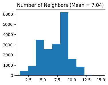
separ.compute_graph()
# Select features using Moran's I
separ.select_morani(nslt=2000)
# Compute weights
separ.compute_weight(n_cluster=10)
After filtering: (19109, 14376)
Counting moran's i ...

Finish selecting
1. Running SEPAR Algorithm
# Run SEPAR algorithm
separ.separ_algorithm(
    r=30,              # Number of spatial patterns
    alpha=0.8,         # Graph regularization weight
    beta=0.05,         # Sparsity penalty weight (previously l1)
    gamma=0.5          # Pattern orthogonality weight (previously lam)
)
Processing iterations: 100%|██████████| 100/100 [02:11<00:00, 1.32s/it]
2. Identifying Pattern-Specific Genes
# Identify pattern-specific genes
pattern_genes = separ.identify_pattern_specific_genes(
    n_patterns=30,    # Number of patterns to consider
    threshold=0.3     # Threshold for gene-pattern association
)
Pattern Visualization and Pattern-specific Genes
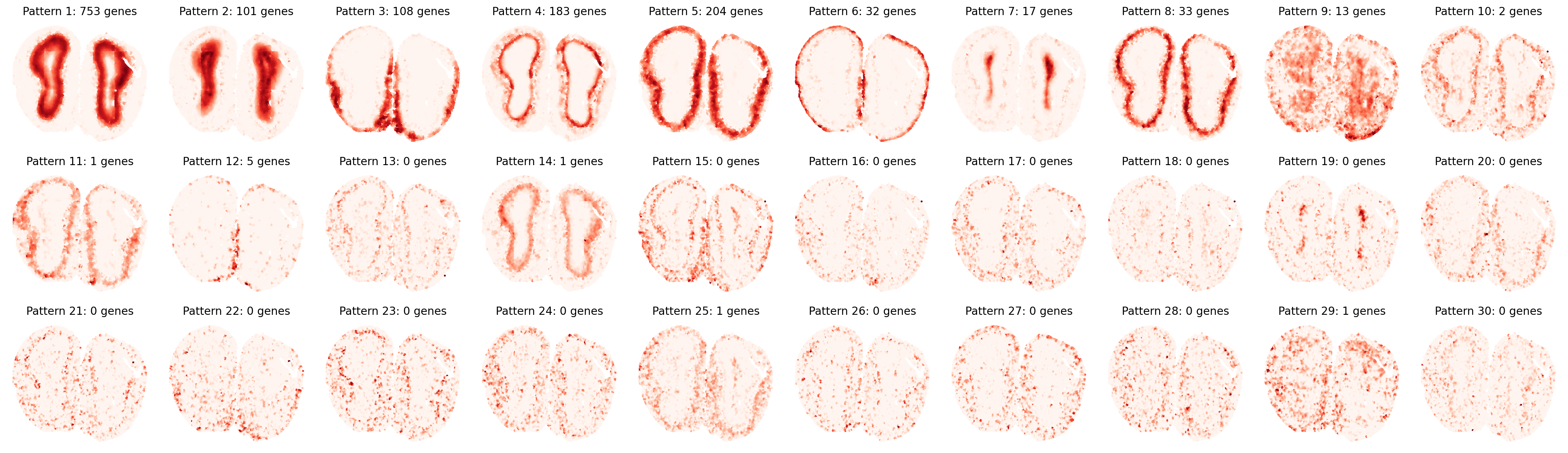
First, let’s visualize the identified spatial patterns and analyze their characteristics:
# Visualize all spatial patterns
sim_slt = separ.sim_res(separ.Wpn, separ.Hpn, separ.Xt.T)
sim_argsort = np.argsort(-sim_slt)

num_patterns = 30
plt.figure(dpi=200, figsize=(24, 7))
for i in range(30):
    ii = sim_argsort[i]
    plt.subplot(3, np.int32(num_patterns/3), i + 1)
    plt.scatter(separ.loc[:, 0], separ.loc[:, 1],
                c=separ.Wpn[:, ii].reshape(-1, 1),
                s=1.2, cmap='Reds')
    plt.axis('off')
    plt.title(f'Pattern {i + 1}: {int(separ.genes_per_pattern[ii])} genes',
              fontsize=12)
plt.tight_layout()
plt.show()
# Create and display sorted pattern-specific genes table
print("\nTop Pattern-Specific Genes (Sorted by Pattern Significance):")
print("-" * 100)
print(f"{'Pattern':11} | {'Significance':11} | {'#Genes':8} | {'Top Genes'}")
print("-" * 100)

for rank, pattern_idx in enumerate(sim_argsort[:30]):
    genes = pattern_genes[pattern_idx]
    if len(genes) == 0:
        gene_str = "None"
    else:
        gene_str = ", ".join(genes[:10])
        if len(genes) > 10:
            gene_str += "..."

    print(f"Pattern {rank+1:<3} | {sim_slt[pattern_idx]:.4f}      | {len(genes):<8} | {gene_str}")
print("-" * 100)
Top Pattern-Specific Genes (Sorted by Pattern Significance):
----------------------------------------------------------------------------------------------------
Pattern     | Significance | #Genes   | Top Genes
----------------------------------------------------------------------------------------------------
Pattern 1   | 0.9338      | 753      | Npas4, Cpne6, Necab3, Egr4, Slc35d3, Hpcal4, Shisa8, Cdkn1a, Fam126a, Dusp14...
Pattern 2   | 0.8867      | 101      | Nrgn, Cartpt, Ctxn3, Prkcg, Dll1, C130073E24Rik, Camk4, Lamp5, Necab2, Gm45341...
Pattern 3   | 0.8674      | 108      | Clca3a1, Agt, Cebpd, Serpina3n, Gm34838, Matn4, Omp, S100a5, Kctd12, Hmgcs2...
Pattern 4   | 0.8625      | 183      | Shisa3, Lbhd2, Kcnk15, Nefm, Nefh, Spp1, Npr1, Tbx21, Lrrtm1, Nrn1...
Pattern 5   | 0.8586      | 204      | Nppa, Trh, AI593442, Cnr1, Calb1, Insm1, Gm11549, Gpx3, Fibcd1, Syndig1l...
Pattern 6   | 0.7912      | 32       | Fmod, Ogn, Nov, Slc6a20a, Slc13a4, Igf2, Mgp, Slc6a13, Col1a2, Aebp1...
Pattern 7   | 0.6884      | 17       | Igfbpl1, Prokr2, Naaa, Carhsp1, Sox11, Mobp, Id4, Prr18, Ednrb, Mbp...
Pattern 8   | 0.6852      | 33       | Barhl2, Cbln4, Cck, Coch, Adcyap1, Olfr115, Tmem40, Nptx1, Mafa, Cdhr1...
Pattern 9   | 0.4574      | 13       | Tmsb4x, Gm3839, Gm32401, Gramd1c, Gm3764, Gm10800, Clec18a, Caps2, Gm33838, Gm16863...
Pattern 10  | 0.4347      | 2        | Vip, Sst
Pattern 11  | 0.3793      | 1        | Palmd
Pattern 12  | 0.3730      | 5        | Hba-a2, Hbb-bt, Hba-a1, Hbb-bs, Acta2
Pattern 13  | 0.2760      | 0        | None
Pattern 14  | 0.2665      | 1        | Nme7
Pattern 15  | 0.2405      | 0        | None
Pattern 16  | 0.2232      | 0        | None
Pattern 17  | 0.2211      | 0        | None
Pattern 18  | 0.1995      | 0        | None
Pattern 19  | 0.1995      | 0        | None
Pattern 20  | 0.1954      | 0        | None
Pattern 21  | 0.1823      | 0        | None
Pattern 22  | 0.1805      | 0        | None
Pattern 23  | 0.1801      | 0        | None
Pattern 24  | 0.1801      | 0        | None
Pattern 25  | 0.1795      | 1        | Cdk8
Pattern 26  | 0.1714      | 0        | None
Pattern 27  | 0.1641      | 0        | None
Pattern 28  | 0.1573      | 0        | None
Pattern 29  | 0.1550      | 1        | Tmsb4x
Pattern 30  | 0.1541      | 0        | None
----------------------------------------------------------------------------------------------------
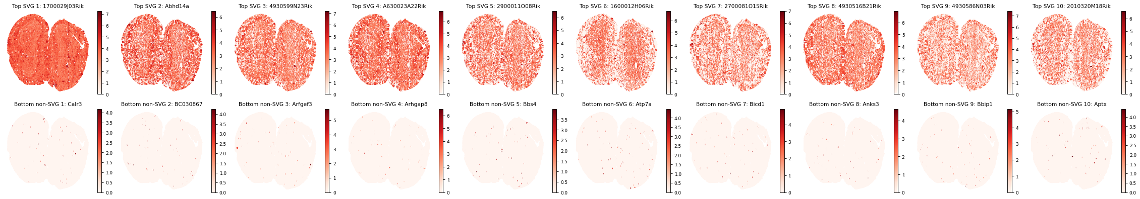
3. Spatially Variable Genes (SVGs) Analysis
# Get SVG results
svg_results = separ.recognize_svgs(err_tol=0.7)
Visualize some top and bottom SVGs:
gene_ranking = svg_results['gene_ranking']
# Create a single figure with subplots for top SVGs and bottom non-SVGs
plt.figure(figsize=(8.5/3*10, 5), dpi=80)
plt.rcParams['font.size'] = 8
# Plot top 10 SVGs
for i in range(10):
    plt.subplot(2, 10, i+1)
    gene_idx = gene_ranking[i]
    gene_name = adata.var_names[gene_idx]
    gene_exp = separ.adata[:, gene_idx].X.toarray().flatten()

    scatter = plt.scatter(separ.adata.obsm['spatial'][:, 0],
                        separ.adata.obsm['spatial'][:, 1],
                        c=gene_exp, s=5, cmap='Reds')
    plt.title(f'Top SVG {i+1}: {gene_name}')
    plt.axis('off')
    plt.colorbar(scatter)

# Plot bottom 10 non-SVGs
for i in range(10):
    plt.subplot(2, 10, i+11)
    gene_idx = gene_ranking[-(i+1)]
    gene_name = adata.var_names[gene_idx]
    gene_exp = separ.adata[:, gene_idx].X.toarray().flatten()

    scatter = plt.scatter(separ.adata.obsm['spatial'][:, 0],
                        separ.adata.obsm['spatial'][:, 1],
                        c=gene_exp, s=5, cmap='Reds')
    plt.title(f'Bottom non-SVG {i+1}: {gene_name}')
    plt.axis('off')
    plt.colorbar(scatter)

plt.tight_layout()
plt.show()
4. Gene Expression Refinement
adata_refined = separ.get_refined_expression()
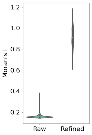
Evaluating Refinement Performance
First, we use Moran’s I statistic to quantitatively evaluate the improvement in spatial patterns. Moran’s I measures spatial autocorrelation, with higher values indicating stronger spatial patterns. The violin plot below compares the distribution of Moran’s I values between raw and refined expression data across all genes:
# Calculate Moran's I for both raw and refined data
morani = sc.metrics.morans_i(separ.adata)
morani_refine = sc.metrics.morans_i(adata_refined)

# Create DataFrame for violin plot
data_violin = pd.DataFrame({
    'Moran\'s I': np.concatenate([morani, morani_refine]),
    'Condition': ['Raw'] * len(morani) + ['Refined'] * len(morani_refine)
})

import seaborn as sns
# Create violin plot
plt.rcParams['font.size'] = 16
plt.figure(figsize=(3, 5.5))
sns.violinplot(x='Condition', y='Moran\'s I', data=data_violin, palette='Set2')
plt.ylabel('Moran\'s I')
plt.xlabel('')
plt.show()
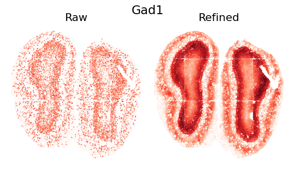
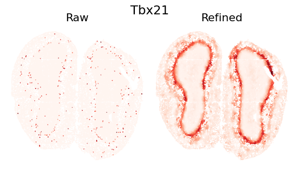
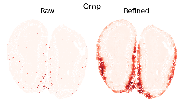
Single Gene Visualization
To demonstrate the refinement effect at individual gene level, we visualize the spatial expression pattern of a single gene. The comparison shows how SEPAR preserves and enhances genuine spatial patterns while reducing technical noise:
def plot_gene_refinement(gene_name, separ, adata_refined):
    """
    Visualize raw and refined expression patterns for a specific gene.

    Parameters
    ----------
    gene_name : str
        Name of the gene to visualize
    separ : SEPAR object
        SEPAR object containing raw data
    adata_refined : AnnData
        Refined expression data from get_refined_expression()
    """
    # Get gene index and expression values
    gene_idx = separ.adata.var_names.get_loc(gene_name)
    raw_exp = separ.adata[:, gene_idx].X.toarray().flatten()
    refined_exp = adata_refined.X[:, gene_idx]

    # Create comparison plot
    plt.rcParams['font.size'] = 16
    plt.figure(dpi=100, figsize=(7/1.2, 4/1.2))

    # Set main title
    plt.suptitle(gene_name, fontsize=18)

    # Plot raw expression
    plt.subplot(1, 2, 1)
    plt.scatter(separ.loc[:, 0], separ.loc[:, 1],
                c=raw_exp, s=0.3, cmap='Reds', rasterized=True)
    plt.axis('off')
    plt.title('Raw', fontsize=16)

    # Plot refined expression
    plt.subplot(1, 2, 2)
    plt.scatter(separ.loc[:, 0], separ.loc[:, 1],
                c=refined_exp, s=0.3, cmap='Reds', rasterized=True)
    plt.axis('off')
    plt.title('Refined', fontsize=16)

    plt.tight_layout(pad=0)
    plt.show()

plot_gene_refinement("Gad1", separ, adata_refined)
plot_gene_refinement("Tbx21", separ, adata_refined)
plot_gene_refinement("Omp", separ, adata_refined)
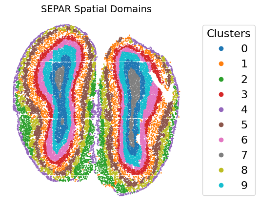
5. Performing Clustering
# Perform clustering
cluster_res = separ.clustering(n_cluster=10, N1=16, N2=4)
Clustering Results Visualization
# Create visualization
fig, ax = plt.subplots(figsize=(6, 5), dpi=100)
scatter = ax.scatter(separ.loc[:, 0], separ.loc[:, 1],
                    c=separ.labelres, s=1, cmap='tab10')
plt.title("SEPAR Spatial Domains", fontsize=14)
plt.axis('off')

# Add legend
legend = ax.legend(*scatter.legend_elements(),
                  title="Clusters",
                  bbox_to_anchor=(1.05, 0.5),
                  loc='center left')

plt.subplots_adjust(right=0.75)
plt.show()
References
[1] Dong, Kangning, and Shihua Zhang. “Deciphering spatial domains from spatially resolved transcriptomics with an adaptive graph attention auto-encoder.” Nature Communications 13.1 (2022): 1-12.